Stochastic Simulations for Dummies: Why Random Motion Needs √(Δt)

Let’s talk about randomness. Not just any randomness—the kind that makes tiny pollen grains jiggle in water (Brownian motion) or stock prices wiggle unpredictably.

Deterministic vs. Random Motion

The Predictable World

Suppose you are moving around with velocity \(v\). How much will you have traveled after a small time \(\Delta t \)? The answer is \(\Delta x= v \Delta t\), provided that the time increment is small enough and the velocity does not change much (is continuous). This makes sense: double the time, double the distance. Today, we will see how randomness breaks this very intuitive scaling - and of course how to remedy this.

The Random World

Now suppose you take random steps—like a drunk person staggering left and right. Each step is independent, and on average, you go nowhere. But you don’t stay perfectly still—you spread out over time. By this I mean if you do this with 100 friends, you expect people to be more spread out over time. So the key ideas are:

• The average position stays zero
• The spread (variance) grows with time. The variance is the average of the square of the distance.

The second of these ideas, the growth of the variance, is critical to properly simulating random motion. We will see the growth of variance is proportional to the time interval, \(\Delta t\). Because the variance is like a squared distance, we are essentially claiming that \(\Delta x^2\approx\Delta t\). Here is our first introduction to the aforementioned scaling, if we solve for \(\Delta x=\sqrt{\Delta t}\). Let’s have a closer look at this.

Why variance grows linearly

Suppose you take $N$ independent random steps of size \(\pm \Delta \), with equal chance for each option. By independent we mean that our previous step does not influence our next step, and if you want to be concrete you can take \(\Delta x=1\) without loss of generality. Suppose we take those steps in \(T\) seconds (or minutes, it does not really matter). Then, each step takes \( \Delta t=T/N\), or more usefully \(N=T/\Delta t\).

Now, if each step is called \(x_{j}=\pm \Delta x\), then our current poition is \(X_N=x_1+\cdots+x_N\). As the average of each step is zero, and the expectation is linear, \(\mathbb{E}(X_N)=0\), i.e. the mean displacement is zero. However, we have to be more careful computing the variance. Because the steps are independent, we can compute the variance of the sum as the sum of the variances (this is in general NOT true and you have to always be careful about this!). For our purposes:

The first step uses independence to write the variance of a sum as the sum of the variances. Because all steps are identical, the variance is the same for all of them, so we just need to compute it for the first one. We can compute the variance (of a random variable \(X\)) using \( \mathrm{Var}(X)=\mathbb{E}(X^2)-\mathbb{E}(X)^2\), where \(\mathbb{E}\) is the expectation. We already figured out the expectation of \(x_1\) is zero, so that the second term is zero. For the first one:

This is because the probability to moving to the right (and to the left) is 0.5. The spread (varaince of \( X_N\)) after \(T\) seconds is thus

Here’s the problem: if we want to take more and more steps and run the simulation for the same time, then \( \Delta t\) get’s smaller and smaller, and the variance blows up. this is undesireable, physics should not break down when we use smaller time steps (excluding quantum effects etc…). in practice, this means we must also make our step size constant. In particular, in order to keep the variance constant as \(\Delta t\rightarrow0\), we must have \(\Delta x^2=\Delta t\). In deterministic physics we usually face a similar problem, but this is usally remedied by using \(\Delta x \sim \Delta t\).

We can already predict some interesting differences from our little analysis. Unlike deterministic motion, if we wait twice as long we do not expect the distance to be twice as large. Instead, for random motion we expect to be \(\sqrt{2}\) as large, which is not as far away as for deterministic motion. Thus, random things are slower.

Let’s simulate some things now.

Some very basic code to simulate the stock market

Suppose a particular stock, or asset, moves up and down like the drunk person from the previous example. Inherently, this means that it is unbiased to really go up or down, because on average it does not move. We will simulate this and see what happens when we use both \(dt\) and \(\sqrt{dt}\) to update our simulation. Here is some python code that simulates random walks, both with the correct and the incorrect scaling:

import numpy as np
import matplotlib.pyplot as plt

def random_walk(T=1, N=500, correct=True):
    dt = T/N
    if correct:
        steps = np.sqrt(dt)*np.random.randn(N)
    else:
        dt*np.random.randn(N)
    return np.cumsum(steps)

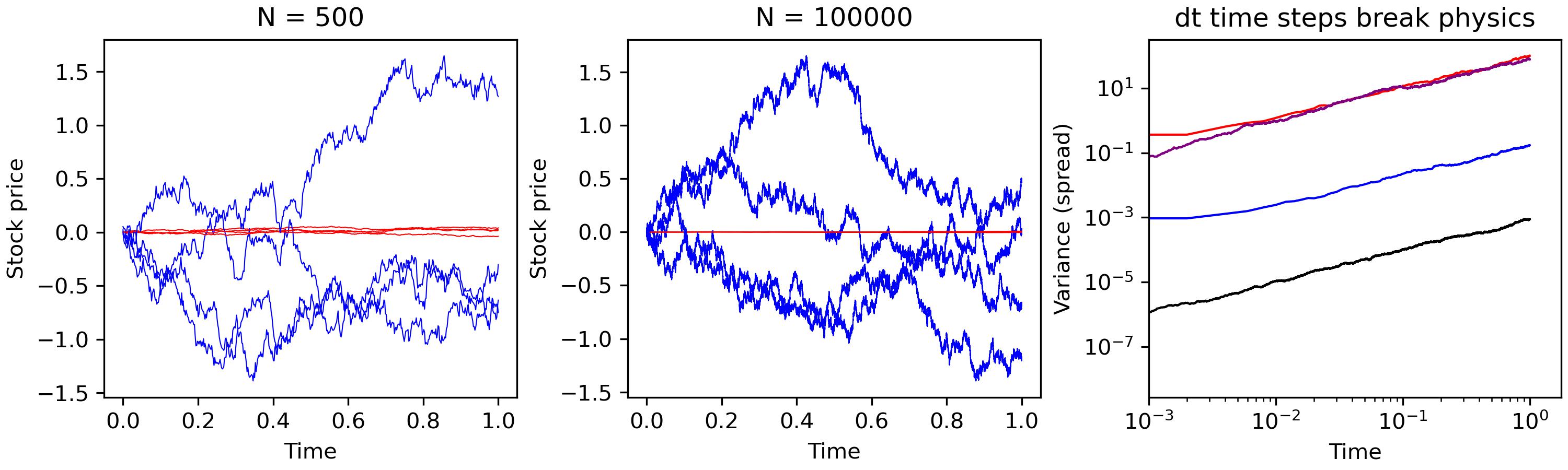
Now, we do the follwing experiment: we run the same simulation a hundred times, for both N=500 and N=10000 time steps. We plot some trajectories for both the correct scaling (blue) and the incorrect scaling (red) in the left (N=500) and middle (N=10000) panels. We see that the blue lines are qualitatevily similar (same order of magnitude), except that the higher resolution simulations have a richer microstructure. The story for the red lines is different: the red lines for N=500 move more than the red lines for \(N=10^4\). We expect thigns to behave simlarly for different step sizes, so we know we must be using the wrong choice for the step size (and we are). The right panel confirms our intuition. We plot the variance (specifically the sum of the squares of the trajectories to the left), as a function of time, for the four cases. The \(\sqrt{dt}\) lines (red and purple) collapse to a single scaling, confirming this is the correct choice. The \(dt\) lines (black and blue) are very different, so this must be the wrong choice.

In the next entries in this series we will see how to generalize some of the ideas presented here. For instance, what shoudl we do if we suspect our stock will go up or down in the long term? What if we want to apply these ideas to simulate flying insects? How can we handle complicated domains? How can we make our code run faster if we need to run many many simulations? Stay tuned!