Modelling extinction events

Starting from the model presented by Frank et. al. in “Investigating Anthropogenic Mammoth Extinction with Mathematical Models”, we will provide some simulations of the ODE system presented for the extinction of mammoths.

In follow up posts, we will generalise their model to include spatial effects, turning it into a PDE system (a continuum version from their grid based apporach). We start with a simplified dimensionless version fo their ODE model

we neglect their migration term, which will be incorporated in the spatial scenario. Here, \( H \) is the number of humans, \( M \) is the number of mammoths. The parameters represent different phenomenological laws: $\alpha$ represents the Alle effect etc…, and the nonlinear coupling is a standard predation term.

The standard approach to study this system is to linearise around equilibria and study their stability by looking at the sign of the eigenvalues of the Jacobian matrix. A summary of the results for this is presented in their paper, and here we opt to perform a limited parameter sweep. First, we provide code to solve the system, using Scipy’s built in integrator and specifying the integration method as RK45. Unlike in other scenarios, this problem is not stiff and we do not require a stiff integrator. With a future parameter sweep in mind, we set up the function with parameters so that it is easily called later.

import numpy as np
import matplotlib.pyplot as plt
from scipy.integrate import solve_ivp

def RHS(t,vector,A_H, B_H, r,alpha, A_M,B_M):
    H = vector[0];M = vector[-1]
    dHdt = A_H*H*(1-H) + B_H*M**2*H/(M**2+r**2)
    dMdt = A_M*M*(1-M)*(alpha*M-1) - B_M*M**2*H/(M**2+r**2)
    return np.array([dHdt,dMdt])

H0=0.1;M0=1
y0 = np.array([H0,M0])
params = {
    'A_H': 1.0, 'B_H': .1, 'A_M': .01, 'B_M': 0.1,'r':.1,'alpha':10
}
T = 20;Nt=300
t_span = (0, T)  # From t=0 to t=10
t_eval = np.linspace(0, T, Nt)
# Solve the PDE system
sol = solve_ivp(
    lambda t, vector: RHS(t, vector, **params),
    [0, T],
    y0,
    t_eval = t_eval,
    method='BDF'
)
H = sol.y[0,:];M = sol.y[-1,:]

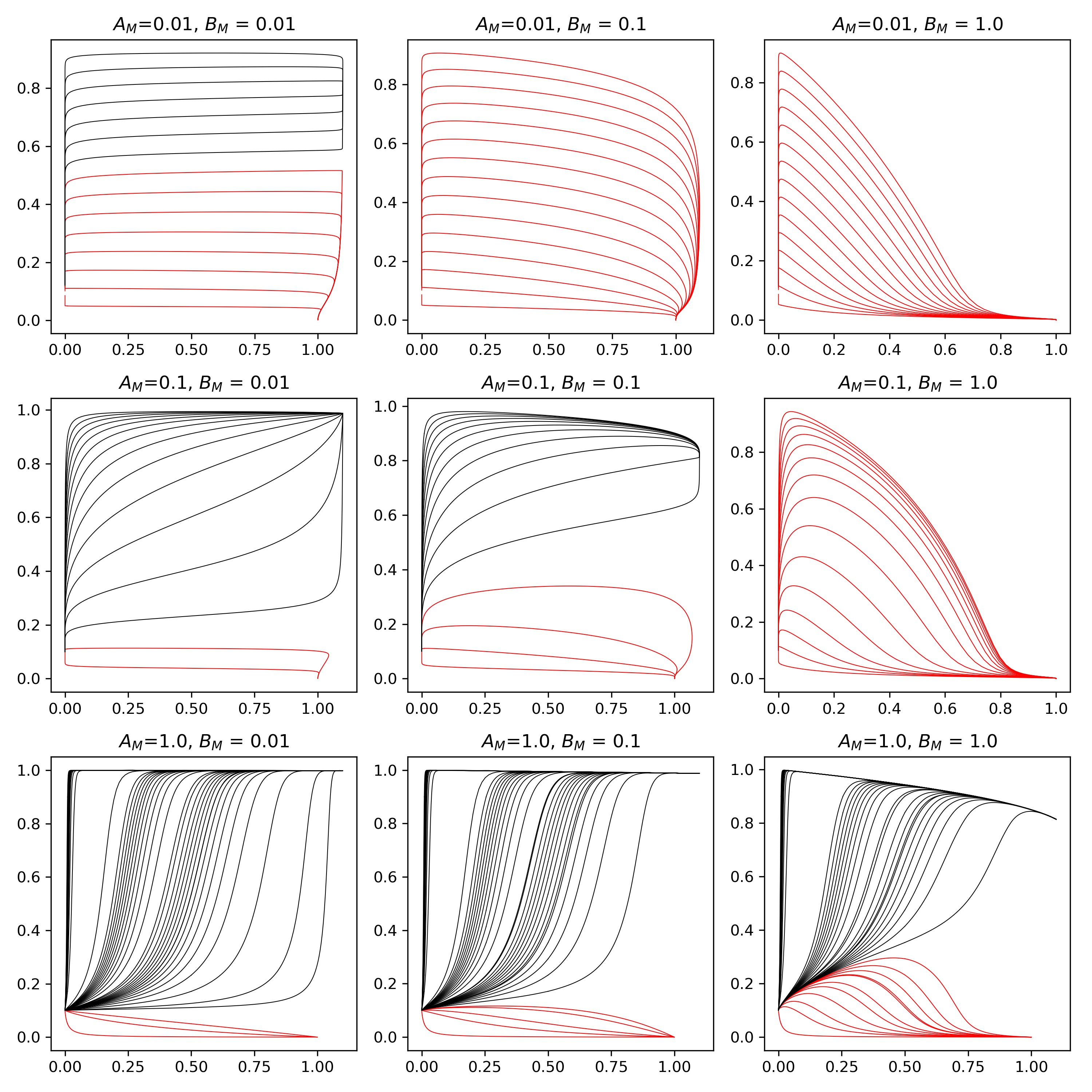
By sweeping through values of the initial conditions and integrating both forwards and backwards in time we can construct phase diagrams, plots in \( (H,M)\) space where we can clearly see the stability of the fixed points.

Here, different values of \(A_M \) and \(B_M \) are represented in the grid.